Project Presentation #
I completed this project at the end of the first semester of my first year in engineering school. The goal was to apply our knowledge of applied mathematics, particularly in probability and statistics, to a real-world case. Our team of four worked on this project for two weeks.
The project focused on the statistical analysis of degradation data. For certain systems, knowing the date of a future failure to anticipate maintenance can be of critical importance. This could be due to high replacement costs or the severe consequences of a failure, such as the collapse of the Genoa Bridge in Italy in 2018. The final objective was to model the degradation level of a system using collected data and then predict the date when a predefined critical threshold would be crossed.
Methodology #
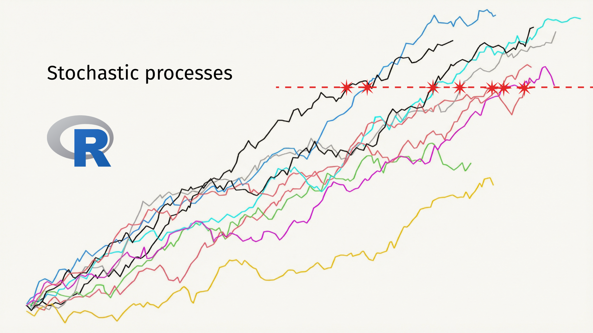
To model the failure level of systems, the natural tool is the use of stochastic processes. A stochastic process describes the evolution of a phenomenon over time, where the path depends, in part, on randomness. During our project, we used two types of processes: the Gamma process and the Wiener process. The Gamma process models strictly increasing evolution (its increments follow a Gamma distribution). The Wiener process, on the other hand, models a level that can either decrease or increase (its increments follow a normal distribution). This process is well-known in finance and physics as it models Brownian motion. We considered these processes in their homogeneous form, meaning with stationary increments (the distribution of increments does not change over time). They are defined by parameters controlling drift and diffusion for the Wiener process, and shape and rate for the Gamma process.
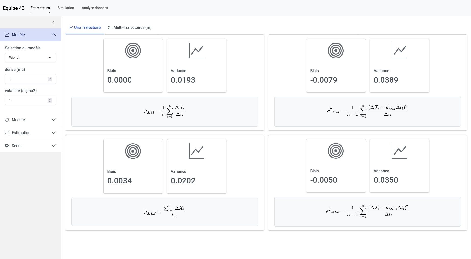
The key task was to estimate these parameters to model failure using the data. Our first major task was to develop estimators to determine the parameter values from empirical observations. We were keen to do this work ourselves to fully understand the methods used, in our case, the method of moments and maximum likelihood estimation, but we also relied on certain references12. For each estimator we derived, it was essential to assess its quality (bias and variance). To do this, we used empirical methods with simulations programmed in the R language.
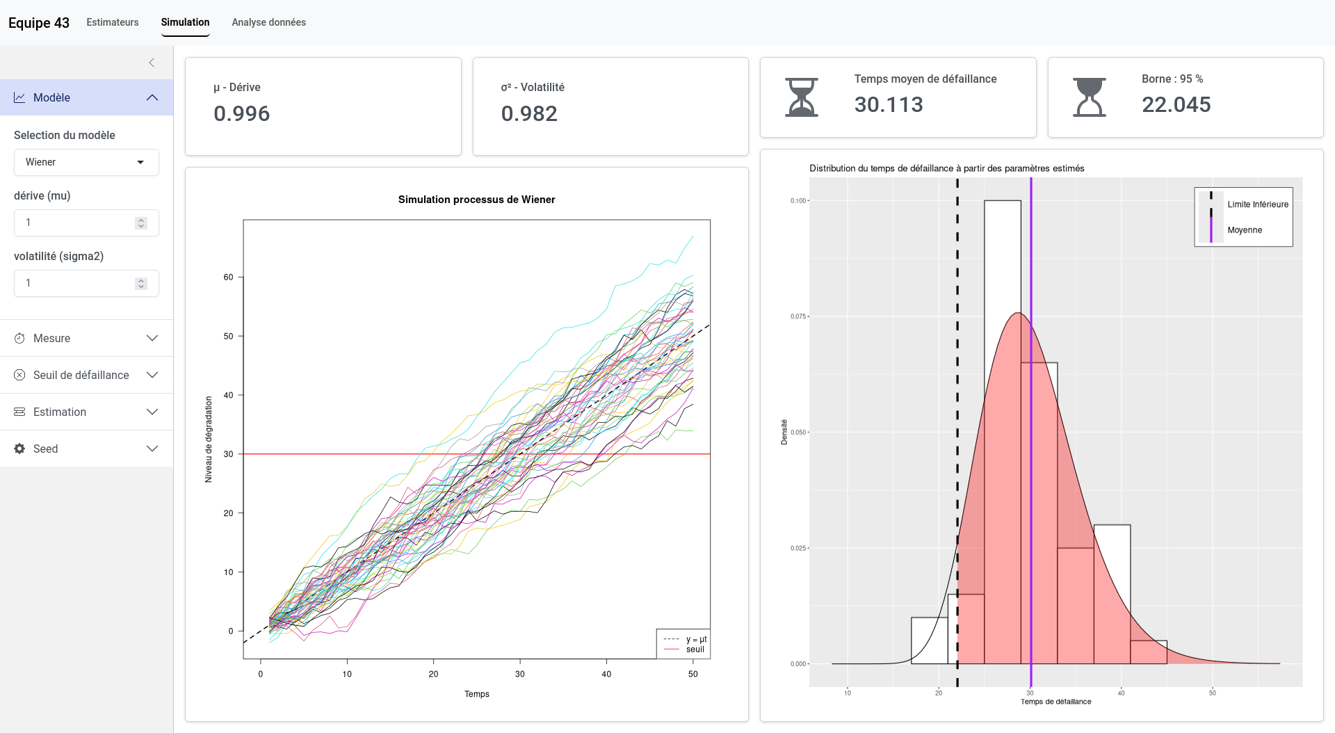
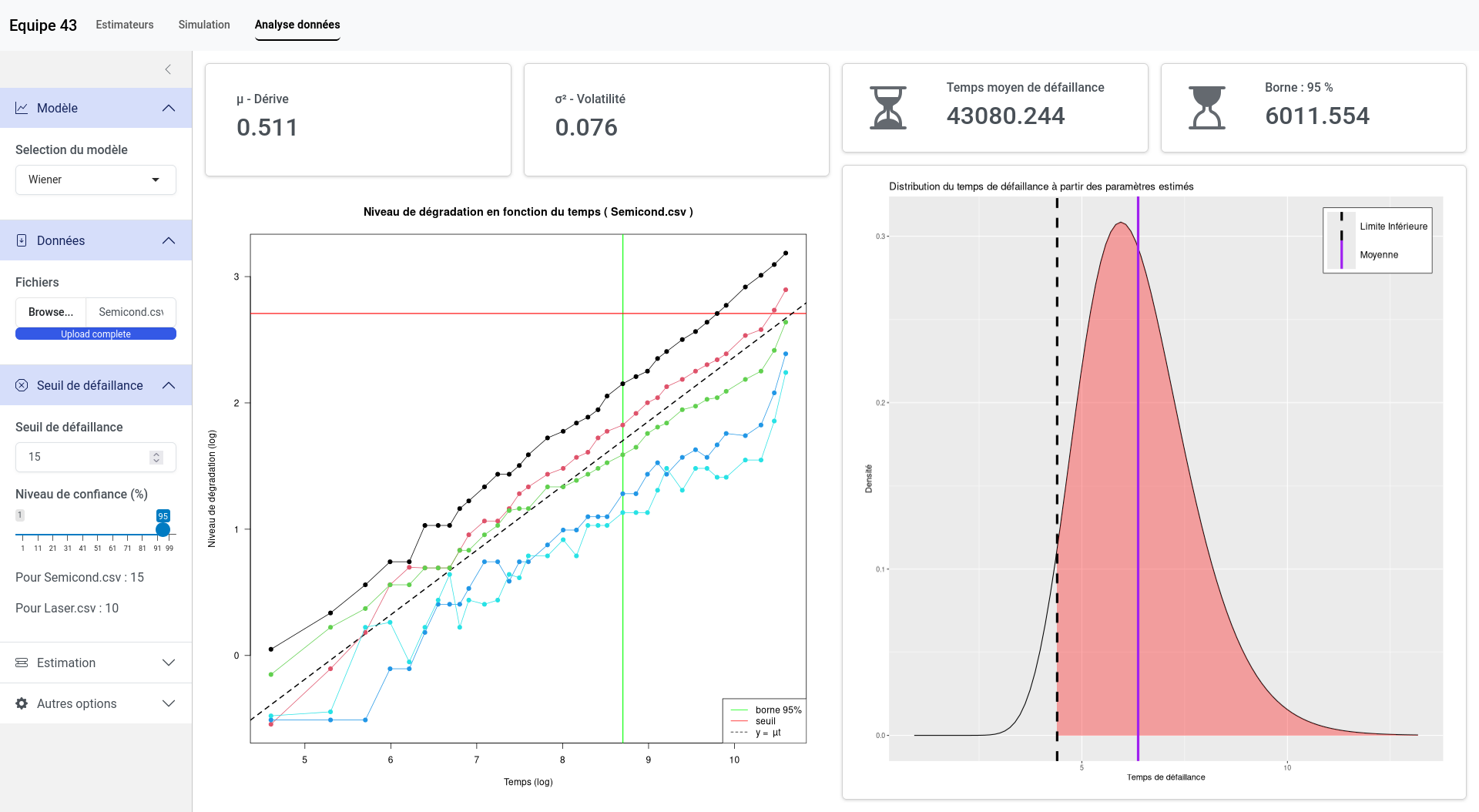
Once we were able to model the degradation processes, the next step was to predict the time to failure. The time at which the threshold is crossed follows a specific probability distribution. For example, in the case of a Wiener process, it follows an inverse Gaussian distribution. Using this distribution, we could calculate the mean time to failure, as well as a lower bound representing a date before which 95% of failures occur. This is particularly useful for preventive maintenance planning.
Finally, the last step of our work involved analyzing two datasets provided to us. The first dataset concerned the degradation of semiconductors due to hot carriers, which is a progressive wear caused by the repeated impact of highly energetic charge carriers inside the transistor. The second dataset focused on lasers, where the degradation indicator was the operating current required to maintain a constant light output. We applied our models to these datasets, but some adaptations were necessary to validate the model assumptions. For example, with the semiconductors, we used a log-log scale to ensure a linear trend and performed a data translation to avoid negative values.
Results #
Over these two weeks, I learned a great deal about statistical analysis methods and stochastic models. Overall, the project was a success, and we delivered relevant results along with a strong grasp of the modeling methodology.
Another crucial aspect was the requirement to design an application to visualize, simulate, and reproduce all the modeling steps. We developed a web application using the Shiny library in R. Its features include:
- Fully customizable simulation of Wiener and Gamma processes,
- Testing the quality of estimators through simulation,
- Customizable analysis of a dataset.
At the end of our project, we began exploring more complex models using non-homogeneous Wiener processes. In these models, the increments no longer follow a normal distribution \(\mathcal{N}(\mu\Delta t, \sigma^2 \Delta t)\), but rather \(\mathcal{N}(\mu(\Delta t)^{\alpha}, \sigma^2 \Delta t)\). We successfully estimated the parameters of this type of process using maximum likelihood estimation and linear regression. However, we did not have time to apply it to our datasets. Further explorations were possible, such as using non-homogeneous Gamma processes or modeling Wiener processes with imperfect maintenance.